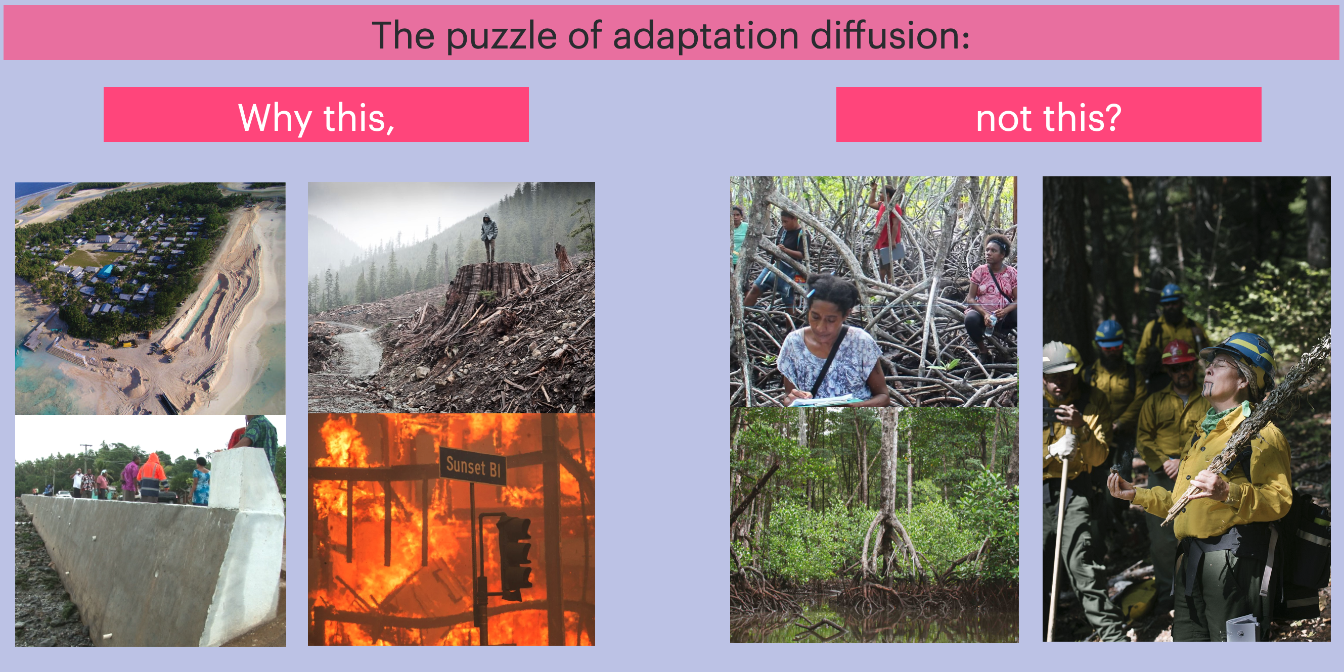
Indigenous, local peoples of the South Pacific Islands and other coastal habitats have sustainably managed mangrove forests to dissipate storm surges and prevent erosion, mitigating potential costs of climate change since long before the anthropocene (Alongi 2002; Nalau et al. 2018; Pearson, McNamara, and Nunn 2020; McNamara et al. 2020). First peoples of western North America have similarly practiced prescribed burns to prevent destructive wildfires during times of drought for millennia (Eisenberg et al. 2019; Kolden 2019). Despite their long-known effectiveness, adaptive practices like these often fail to spread widely. Instead, international development agencies frequently advocate for the construction of seawalls, for example, even though seawalls can exacerbate flooding once breached and incur high maintenance costs (Piggott-McKellar et al. 2020). Inland forest management is beset by polarization among stakeholders (Swette, Huntsinger, and Lambin 2023), resulting in devastating wildfires burning a buildup of fuels or greenhouse gas-intensive clearcuts.
Here we introduce what we dub the puzzle of diffusion: why do some effective, sustainable practices like mangrove forest management fail to diffuse broadly, while other less effective or even maladaptive practices become widespread (Figure 1.1)? To answer this, we answer some more basic questions along the way. First, how do people decide what to do, i.e., how does learning work? Second, what is the effect of identity on how well or how likely we are to learn from people of the same or different identity? Third, what is the effect of social structure, i.e., who knows whom, represented as a social network? Agent-based models are useful because they provide a framework for creating rigorous, mechanistic, concrete models of social diffusion of adaptations. They help us deal with the complexity of causation in the real world through strategic selection of causal input variables and model details, which, over several model time steps, lead to social emergent phenomena like the diffusion of climate change adaptations.
The focus of this course is developing agent-based models that can help us simplify complex combinations of cognitive and social factors to represent only the most relevant ones, and observe the effect of these on simulated outcomes such as the proportion of people adopting adaptive behaviors, or opinion extremism and polarization.
Why agent-based models are useful
Agent-based models (ABMs) provide a structured way to explore complex systems by simulating interactions between autonomous agents, i.e., simulated people. In sustainability contexts, ABMs offer a low-cost testbed for understanding how interventions might impact social dynamics and environmental outcomes. For example, Airoldi and Christakis (2024) demonstrated through regression analysis across that one method for selecting individuals targeted in a public health education campaign worked better than another. They studied over 20,000 individuals across Honduran villages of about 100 people each to reach their findings. Real-world verification of the efficacy of different intervention strategies is important. However, we can also use agent-based models to represent the diffusion of information in simulated populations where interactions are structured by model social networks. We can initialize thousands or millions of simulated villages in which this information could diffuse with different intervention strategies, and observe the distribution of the adoption of sustainable behaviors for each potential intervention strategy. We can then analyze which performed best in silico, which can be helpful if interventions will be taken to different contexts. In other worlds, we can use ABMs to deduce how different learning rules, group identities, and social structures shape sustainability outcomes generally, which can guide our selection of real-world intervention strategies.
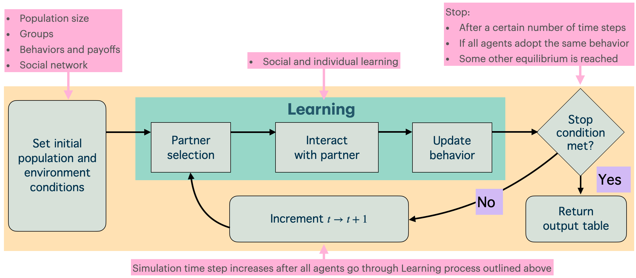
A typical ABM simulation cycle includes (Figure 1.2):
- Initializing agent populations and environmental conditions
- Iterative steps where agents select partners, interact, and update behaviors based on outcomes and learning rules
- Repeating these steps until specific conditions or thresholds are met
- Generating output data for analysis
We will analyze and draw on several real-world empirical studies of interventions to develop our agent-based models that we in turn will use to simulate interventions in order to deduce which strategies are most effective for social interventions to promote sustainability, and why. A social intervention (or just intervention) for promoting sustainability is any concerted effort where those promoting a sustainable practice introduces information about how to perform that practice to a population. Deductive methods complement regression-based inferential or inductive strategies. Deductive strategies can explain which strategies are most effective and why in idealized, cost-free settings (cost-free at least compared to the cost of real-world social interventions at scale).
Low-cost experimentation with simulated social interventions to promote sustainability are critical. Unless progress is accelerated towards we can expect to “have 575 million people living in extreme poverty, 600 million people facing hunger, and 84 million children and young people out of school. Humanity will overshoot the Paris climate agreement’s 1.5°C ‘safe’ guardrail on…temperature rise. And, at the current rate, it will take 300 years to attain gender equality” (Malekpour et al. 2023, 250). Accelerated transformations are required to reach goals necessary to avoid increasingly frequent and costly climate change disasters (United Nations 2023). It is not plausible to do real-world experiments at the global scale required to infer which strategies work best in which situations.
In this course we will focus on deducing how between different cognitive and social factors, or other initial conditions, affect simulated sustainability intervention outcomes. We will frame our studies in terms of sustainable development goals, but we will never fit our models to observations. Nonetheless, we will strive to develop models that are amenable to real-world interventions against which the models could be fit and predictions could be compared. It seems this is not done too much in practice yet in sustainability. However, some of our colleagues focused on studying basic processes that underlie cultural transmission do exactly this to explain experimental data and archaeological observations (Deffner et al. 2024), which thereby improves their theory, models, and understanding of cultural evolution in a theory-model-observation cycle. With more time and research effort, this cycle may become commonplace in sustainability.
The urgent need to understand how sustainable behaviors spread in order to develop effective interventions pressures social scientists to make social science more rigorous, reliable, and digestible by non-social scientists. In the rest of this Introduction we review cognitive and social theories of social learning, identity and influence, homophily and core-periphery network structures, and preview the remainder of the course material. For an overview of the course feel free to skip ahead to the Plan in table format.
Social learning strategies
Human kind is set apart by powerful learning and reasoning capabilities (Witt et al. 2024) that enable cultural transmission and accumulation of technologies and practices no other species matches (Henrich 2015). For our sustainability models, we only need simple models of cognition and learning. It would never be practical to do psychological or cognitive tests in the context of sustainability interventions that targets large populations, for one thing, so we could never compare detailed cognitive assumptions or predictions with reality. For our purposes we will consider three general classes of learning strategy:
- Success-biased learning: Individuals are more likely to adopt behaviors perceived to be successful or beneficial.
- Frequency-biased learning: Individuals adopt behaviors because others are already doing them, creating a conformity effect.
- Contagion: Individuals copy behaviors simply by observing others performing them.
In the mangrove versus seawall example, success-biased learning might favor seawalls if influential external actors, who seem successful or wealthy, advocate for them, even if seawalls are ultimately less effective. Mangrove forests might become widely adopted if, on the other hand, frequency-biased learning predominates and many communities have adopted that method.
Formal social learning models with example
To make this more concrete, we formalize (i.e., give formulas for) these three learning strategies as follows using the example in Figure 1.3. In the example, there is one focal agent who is the one doing the observing/learning, labelled with the ID 1, and three social network neighbors with IDs 2, 3, and 4. The focal agent is deciding whether or not to install residential solar. One of his neighbors has installed it, 2. Based on 1’s perception, 2 is the wealthiest, represented by four dollar symbols. 3 is perceived to have one dollar and 4 has two dollars.
Success-biased learning
In success-biased learning, learners first choose an interaction partner/teacher randomly weighted by observed fitness of their neighbors, which is a generic term for wealth, power, status, etc. In general for this case, the probability that learner \(i\) chooses teacher \(j\) is
\[
\Pr(i \text{ chooses } j) = \frac{f_j}{\sum_{k \in n_i} f_k}.
\]
The probability that \(i\) adopts \(A\) is then the sum of the probabilities of choosing each neighbor performing \(A\) (contained in the set \(m_i\)),
\[
\Pr(i \text{ adopts } A) = \frac{\sum_{j \in m_i} f_j}{\sum_{k \in n_i} f_k}.
\]
In our example, only one neighbor installed residential solar with a fitness (i.e. wealth in this example) of 4, while the others have finess 1 and 2. Therefore, \(\Pr(1 \text{ adopts } A) = \frac{4}{7}\).
Frequency-biased learning
In frequency-biased learning there is no interaction partner or teacher chosen. The probability of adoption is only given by the relative frequency of each behavior. The general expression is
\[
\Pr(i \text{ adopts } A) = \frac{|m_i|}{|n_i|}.
\]
In our example, then, the probability of installing residential solar under frequency-biased learning is \(\frac{1}{3}\).
Contagion learning
In the contagion learning model, the focal agent’s (i.e., the learner’s) teacher (i.e., interaction partner) is chosen at random. Then, the learner adopts the teacher’s behavior with probability \(\alpha\), the adoption rate. In this case, then, the probability that 1 adopts residential solar is
\[
\Pr(1 \text{ adopts solar}) = \alpha \Pr(1 \text{ selects 2 as teacher}) = \alpha \frac{1}{3}.
\]
More generally, for focal agent \(i\) with the set of neighbors \(n_i\) (\(n_1 = \{2, 3, 4\}\) in the example), where \(m_i\) is the set of neighbors who have adopted the adaptive behavior (\(m_i = \{2\}\) in the example). We call the adaptive behavior \(A\). The general probability of adoption in contagion learning is therefore
\[
\Pr(i \text{ adopts } A) = \frac{\alpha |m_i|}{|n_i|},
\]
where the \(| \cdot |\) operator counts the number of elements in a set.
Combinations of learning models
There is no reason different learning models cannot be combined. The software we will use in this class, socmod, provides flexibility to the user to define their own learning models. The simplest combination of the three learning models above is to add an adoption rate to either frequency- or success-biased learning. In this approach, one could call the behavior selected by the models above could be considered prospective or candidate behavior to learn, then is actually learned with probability \(\alpha\).
For another potentially useful modification, \(\alpha\) could be defined at the individual level, say \(\alpha_i\), or for dyads (i.e., a pair of interacting individuals) , \(\alpha_{ij}\), where \(i\) is still the focal agent learner, but we have added \(j\), representing the selected teacher.
Identity and Influence
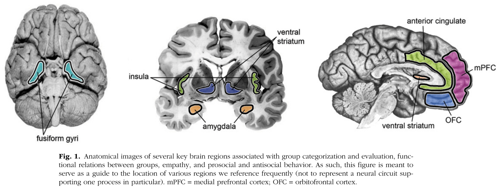
Group identity critically influences social learning. Neuroscience research demonstrates that our brains distinctly respond to individuals identified as part of our group (Cikara and Van Bavel 2014), as revealed through fMRI neural imaging (Figure 1.4). This ability likely evolved because when humans first emerged about two million years ago, it was much more important for survival to be able to rapidly identify whether someone was a friend or foe based on group markers. Although group membership can affect how we respond to information learned from others, group membership itself is quite plastic, meaning who belongs to which group can be rapidly reconfigured. For example, neural signals of race-based group perception was observed to be suppressed and overridden when individuals were in mixed-race groups created by experimenters that competed against other mixed-race groups in an psychological experimental task (Van Bavel, Packer, and Cunningham 2008).
Studies further show that group identity can strongly influence behavioral choices. For instance, experimental evidence reveals people resist adopting beneficial behaviors if associated with opposing political identities (Ehret et al. 2022), emphasizing how identity can create substantial barriers to sustainability. This general effect of group membership interfering with learning is called outgroup aversion (Smaldino et al. 2017).
Social networks, homophily, and core-periphery structure
Social structure can significantly impact behavioral diffusion, especially in core-periphery configurations. Core-periphery networks emerge as a response to risk and uncertainty, e.g., in food sharing networks (Ready and Power 2018), so they are hypothesized to also be important in climate change adaptation transmission networks (Jones, Ready, and Pisor 2021). Core-periphery networks can be created by setting appropriate group sizes and homophily levels in homophily network models (Turner et al. 2023) or specifying certain connectivity probabilities to the stochastic block matrix algorithm for creating structured random graphs (Rombach et al. 2014; Milzman and Moser 2023). Homophily is the measure of how much more likely an individual is to socially connect within their own group versus with a member of a different group. Homophily can range from -1 to +1, where -1 represents no within-group connections and only between-group connections (i.e., anti-homophily); 0 represents an equal probability of within- and between-group connections, and +1 represents only within-group connections. We will define homophily as either a global or group-level variable, though homophily could vary individually as well. There are two types of homophily:
- Choice Homophily: Individuals actively prefer interacting with similar others.
- Induced Homophily: Social interactions limited by historical or external conditions like geography, profession, birthplace, etc.
These structural elements can significantly limit the diffusion of sustainable practices from peripheries, like the mangrove management on smaller islands, to central cores. However, as colleagues and I have showed, this core-periphery structure, defined by moderately high majority-group homophily can actually promote the diffusion of adaptations, provided the adaptation is practiced by the minority group (Turner et al. 2023), as is the case for mangrove forest management or prescribed burns. Formal definitions of homophily and core-peripheriness will be given in the networks chapter.
Course outline in the context of sustainable development
The agent-based modeling approach developed in this course provides a structured way to test the effectiveness of social interventions aimed at promoting sustainable behavior. By formalizing and testing our assumptions about social dynamics, agent-based modeling supports better design and evaluation of policies and programs aimed at driving real-world change. This deductive, experimental approach allows us to explore how cooperation, coordination, identity, homophily, and influence affect the likelihood that beneficial behaviors will spread. In the coming chapters and associated problem sets we will analyze social learning of behaviors and social influence of opinions in various contexts.
The goal is to build up a repertoire of agent-based modeling techniques for incorporating different assumptions about how social learning or influence work, whether group structure is important to these processes, and for modeling social network structure. This repertoire can then be applied to sustainability contexts of interest to understand how different sustainability intervention strategies, such as who should learn about sustainable adaptations first in an educational intervention or how best to assist stakeholder deliberations to reduce opinion polarization that can derail collective adaptation. To choose model components wisely requires an understanding of elements of sustainability, cognitive and social science, network science, and software engineering.
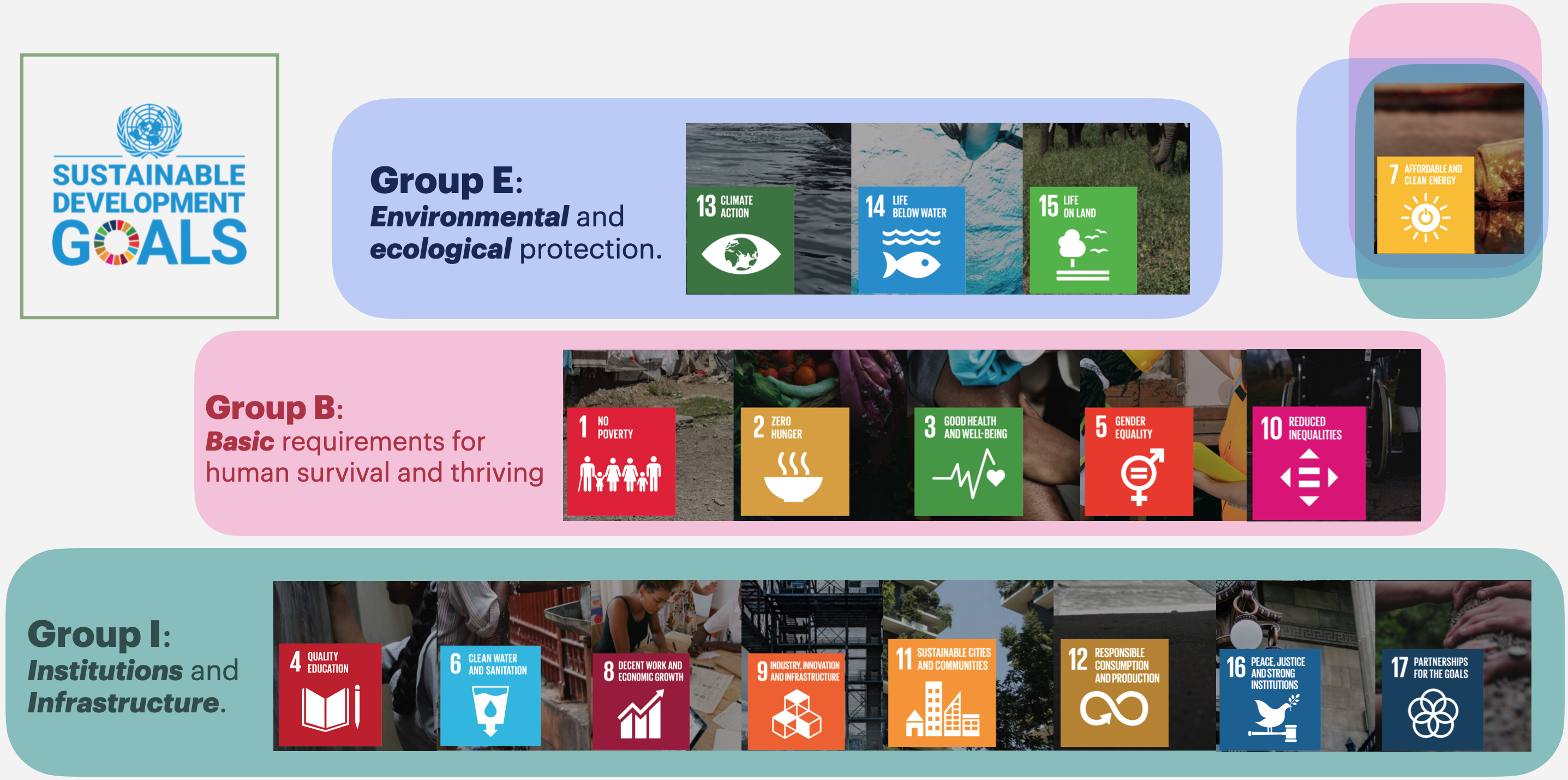
The UN Sustainable Development Goals help us focus and organize our work by providing concrete goals for evaluating progress towards sustainable development for all Figure 1.5. These goals include targets for institutional development that promotes basic conditions for human thriving (justice, equality, education, public health, and no poverty) so as to assemble and enable a critical mass of people to participate bringing about sustainable development. People cannot participate in sustainability if they suffer in poverty, from illness, or subjugation by authoritarians–all but the most zealous environmental defenders will fight on when these basic needs are unmet. Since progress has been slower than necessary.
Sustainability, then, has several different dimensions, all of which contribute to climate action and environmental protection. I have organized these goals into a coding system called the vIBE system: vibrant Institutions support Basic human needs of people who protect the Environment. All 17 goals and the organization system are illustrated in Figure 1.5. Organizing and connecting our work to has two benefits. First, it helps us identify which cognitive and social factors are at work in different sustainability foci. Second, it expands the corpus of existing research on which we draw to consolidate our social and cognitive theories of behavior change that we will apply to sustainability interventions.
Computational social science roots
One goal and theme of socmod is to avoid unneccesary theoretical commitments to either epidemiological forcing-style assumptions (e.g., using SI/SIS/SIR) or to population genetics (e.g., Kimura–Crow models) analyses that represent social learning as evolutionary selection. The agent-based social learning framework provided by socmod accommodates these or other various social behavior models. In the case of diffusion of adaptations, these formalisms share a common mathematical structure of birth–death processes.
We compare these modeling approaches in two ways: first, through their fixation dynamics under weak selection or forcing, and second, through how they each map to a birth–death framework. This is meant to situate users who think in either formalism to how they can map their domain knowledge onto socmod’s framework for agent-based models of social behavior.
Contagion, selection, and social learning
Fixation dynamics arise when a type, trait, or state spreads through a finite population until it completely replaces alternatives. Across epidemiology, population genetics, and social learning, this process can often be formalized using birth–death models, where individuals probabilistically transition between types.
The general structure is:
\[
\frac{dp}{dt} = \text{birth rate} \times (1 - p) - \text{death rate} \times p
\]
where \(p(t)\) is the frequency of the type of interest at time \(t\).
- Birth rate describes how often new instances of the type arise (e.g., infections, successful adoptions, reproductions).
- Death rate describes how often the type is lost (e.g., recoveries, abandonment, replacement by competitors).
In biological contexts, these are referred to as birth–death processes. However, for social learning of adaptive sustainable behaviors, a more accurate description would be learning–unlearning processes: individuals can adopt and later abandon behaviors depending on social influences, network structure, and environmental feedback.
Belief dynamics, which govern the spread and change of internal mental states rather than observable behaviors, differ substantially in mathematical structure. Nonetheless, belief dynamics can also exhibit asymptotic, closed-form approximations under appropriate assumptions.
We focus first on behavioral diffusion processes grounded in social learning. Belief dynamics and their distinct formal properties will be introduced and analyzed in the second part of this book.
In this section, we compare how fixation arises under weak selection or weak forcing in three domains: forcing models from epidemiology, population genetics models, and agent-based social learning models.
Formal Models: Forcing, Genetic Drift, and Success Bias
In epidemiology, the spread of an infectious disease through a population can be captured by systems of ordinary differential equations (ODEs). For a simple SIS (Susceptible–Infected–Susceptible) model, the equations are:
\[
\frac{dS}{dt} = -\beta S I + \gamma I
\] \[
\frac{dI}{dt} = \beta S I - \gamma I
\]
where: - \(S(t)\) and \(I(t)\) are the proportions of susceptible and infected individuals at time \(t\), - \(\beta\) is the transmission rate, - \(\gamma\) is the recovery rate.
Fixation of the infection (i.e., the infected state reaching \(I=1\)) occurs when transmission outpaces recovery, roughly when \(\beta S > \gamma\). In small populations, stochastic drift also matters, especially when \(I\) is small.
In population genetics, the probability of fixation of a new mutant allele can be approximated using Kimura and Crow’s theory. In the simplest form under weak selection:
\[
\text{Fixation probability} \approx p_0 + s(1 - p_0)
\]
where: - \(p_0\) is the initial frequency of the mutant allele, - \(s\) is the selection coefficient (small positive or negative).
In neutral drift (\(s=0\)), the fixation probability equals \(p_0\). When selection is weak but nonzero, the probability is shifted slightly toward the fitter allele.
In social learning models, especially those employing success-biased learning, the analogy to selection is direct. Agents are more likely to copy behaviors that have produced higher payoffs or success in the recent past. This introduces a selection-like bias in the replication of behaviors:
- Drift corresponds to random copying without regard to success.
- Selection corresponds to biased copying favoring higher-payoff behaviors.
Thus, success-biased social learning is mathematically analogous to weak selection in evolutionary models: both introduce a systematic force that, over time, increases the frequency of advantageous types.
Fixation with Weak Selection or Forcing
| Entities |
Susceptible/infected states |
Alleles at genetic loci |
Behaviors or traits in agents |
| Dynamics |
Infection spread vs. recovery |
Reproduction with drift and weak selection |
Social learning with drift and weak biases |
| Fixation driver |
Transmission \(\beta\) overcoming recovery \(\gamma\) |
Drift plus selection (fitness differences) |
Drift plus learning biases (e.g., success or frequency bias) |
| Fixation probability (neutral) |
Equals initial infection fraction |
Equals initial allele frequency \(p_0\) |
Equals initial behavior frequency |
| Fixation probability (with weak selection) |
Infection fixates if \(\beta > \gamma\) |
Approx. \(p_0 + s(1-p_0)\) for small selection \(s\) |
Behavior slightly favored by payoff advantage |
| Time to fixation |
Rapid if \(\beta \gg \gamma\); stochastic early otherwise |
Slow if drift dominates; scales with \(N\) |
Faster with strong bias; scales with network size |
| Role of stochasticity |
Important early, less so later |
Dominant under weak selection |
Dominant under weak learning biases |
| Modeling framework |
Stochastic/deterministic ODEs (SIS, SIR) (Keeling and Rohani 2008; Anderson and May 1991) |
Wright–Fisher, Moran, diffusion approximations (Crow and Kimura 1970; Kimura 1962) |
Agent-based simulations with probabilistic rules (Boyd and Richerson 1985; Rogers 2003) |
- Forcing models focus on infection and recovery dynamics.
- Population genetics tracks allele frequency changes via drift and selection.
- Social learning models behavioral adoption via social influence and drift.
Birth–Death Process Mapping
| Forcing Models (epidemiology, SIS/SIR) |
Infection (Susceptible \(\to\) Infected) |
Recovery (Infected \(\to\) Susceptible) |
| Population Genetics (Kimura–Crow) |
Allele reproduction (fitness-dependent) |
Allele loss (death or replacement) |
| Social Learning (socmod) |
Behavior adoption (social copying or bias) |
Behavior loss or switching |
All three systems feature: - Birth: growth of a type or trait. - Death: loss or replacement. - Drift and bias: stochastic fluctuations and directional forces.
socmod framework for many models
socmod models, by tuning parameters such as success bias, frequency bias, transmission, and dropout rates, can replicate the core behaviors of both population genetics and epidemiology.
Key parallels: - Strong success bias \(\leftrightarrow\) strong selection. - Random copying \(\leftrightarrow\) neutral drift. - Contagion learning \(\leftrightarrow\) stochastic infection.
Thus, socmod models offer a flexible platform bridging epidemiology, evolutionary biology, and social dynamics.
Airoldi, Edoardo M., and Nicholas A. Christakis. 2024.
“Induction of social contagion for diverse outcomes in structured experiments in isolated villages.” Science 384 (6695).
https://doi.org/10.1126/science.adi5147.
Alongi, Daniel M. 2002.
“Present state and future of the world’s mangrove forests.” Environmental Conservation 29 (3): 331–49.
https://doi.org/10.1017/S0376892902000231.
Anderson, R. M., and R. M. May. 1991. Infectious Diseases of Humans: Dynamics and Control. Oxford University Press.
Boyd, R., and P. J. Richerson. 1985. Culture and the Evolutionary Process. University of Chicago Press.
Cikara, Mina, and Jay J. Van Bavel. 2014.
“The Neuroscience of Intergroup Relations: An Integrative Review.” Perspectives on Psychological Science 9 (3): 245–74.
https://doi.org/10.1177/1745691614527464.
Crow, J. F., and M. Kimura. 1970. An Introduction to Population Genetics Theory. Harper; Row.
Deffner, Dominik, Natalia Fedorova, Jeffrey Andrews, and Richard McElreath. 2024.
“Bridging theory and data: A computational workflow for cultural evolution.” Proceedings of the National Academy of Sciences of the United States of America 121 (48): 1–11.
https://doi.org/10.1073/pnas.2322887121.
Ehret, Sönke, Sara M. Constantino, Elke U. Weber, Charles Efferson, and Sonja Vogt. 2022.
“Group identities can undermine social tipping after intervention.” Nature Human Behaviour.
https://doi.org/10.1038/s41562-022-01440-5.
Eisenberg, Cristina, Christopher L. Anderson, Adam Collingwood, Robert Sissons, Christopher J. Dunn, Garrett W. Meigs, Dave E. Hibbs, et al. 2019.
“Out of the Ashes: Ecological Resilience to Extreme Wildfire, Prescribed Burns, and Indigenous Burning in Ecosystems.” Frontiers in Ecology and Evolution 7 (November): 1–12.
https://doi.org/10.3389/fevo.2019.00436.
Henrich, Joseph. 2015. The secret of our success. Princeton University Press.
Jones, James Holland, Elspeth Ready, and Anne C. Pisor. 2021.
“Want climate-change adaptation? Evolutionary theory can help.” American Journal of Human Biology 33 (4): 1–17.
https://doi.org/10.1002/ajhb.23539.
Keeling, M. J., and P. Rohani. 2008. Modeling Infectious Diseases in Humans and Animals. Princeton University Press.
Kimura, M. 1962. “On the Probability of Fixation of Mutant Genes in a Population.” Genetics 47 (6): 713–19.
Kolden, Crystal A. 2019.
“We’re not doing enough prescribed fire in the western united states to mitigate wildfire risk.” Fire 2 (2): 1–10.
https://doi.org/10.3390/fire2020030.
Malekpour, Shirin, Cameron Allen, Ambuj Sagar, Imme Scholz, Åsa Persson, Jaime J. Miranda, Therese Bennich, et al. 2023. “What scientists need to do.” Nature 621 (September): 250–54.
McNamara, Karen E., Rachel Clissold, Ross Westoby, Annah E. Piggott-McKellar, Roselyn Kumar, Tahlia Clarke, Frances Namoumou, et al. 2020.
“An assessment of community-based adaptation initiatives in the Pacific Islands.” Nature Climate Change 10 (7): 628–39.
https://doi.org/10.1038/s41558-020-0813-1.
Milzman, Jesse, and Cody Moser. 2023.
“Decentralized core-periphery structure in social networks accelerates cultural innovation in agent-based model.” In
Proc. Ofthe 22nd International Conference on Autonomous Agents and Multiagent Sys- Tems (AAMAS 2023).
http://arxiv.org/abs/2302.12121.
Nalau, Johanna, Susanne Becken, Johanna Schliephack, Meg Parsons, Cilla Brown, and Brendan Mackey. 2018.
“The role of indigenous and traditional knowledge in ecosystem-based adaptation: A review of the literature and case studies from the Pacific Islands.” Weather, Climate, and Society 10 (4): 851–65.
https://doi.org/10.1175/WCAS-D-18-0032.1.
Pearson, Jasmine, Karen E. McNamara, and Patrick D. Nunn. 2020.
iTaukei Ways of Knowing and Managing Mangroves for Ecosystem-Based Adaptation. Springer International Publishing.
https://doi.org/10.1007/978-3-030-40552-6_6.
Piggott-McKellar, Annah E, Patrick D Nunn, Karen E McNamara, and Seci T Sekinini. 2020.
“Dam(n) Seawalls: A Case of Climate Change Maladaptation in Fiji.” In
Managing Climate Change Adaptation in the Pacific Region, edited by W. Leal Filho, 69–84. Springer.
https://doi.org/10.1007/978-3-030-40552-6.
Ready, Elspeth, and Eleanor A. Power. 2018.
“Why wage earners hunt: Food sharing, social structure, and influence in an arctic mixed economy.” Current Anthropology 59 (1): 74–97.
https://doi.org/10.1086/696018.
Rogers, E. M. 2003. Diffusion of Innovations. 5th ed. Free Press.
Rombach, M. Puck, Mason A. Porter, James H. Fowler, and Peter J. Mucha. 2014.
“Core-periphery structure in networks.” SIAM Journal on Applied Mathematics 74 (1): 167–90.
https://doi.org/10.1137/120881683.
Smaldino, Paul E, Marco A Janssen, Vicken Hillis, Jenna Bednar, Paul E Smaldino, Marco A Janssen, Vicken Hillis, and Jenna Bednar. 2017.
“Adoption as a social marker: Innovation diffusion with outgroup aversion.” The Journal of Mathematical Sociology 41 (1): 26–45.
https://doi.org/10.1080/0022250X.2016.1250083.
Swette, Briana, Lynn Huntsinger, and Eric F. Lambin. 2023.
“Collaboration in a polarized context: lessons from public forest governance in the American West.” Ecology and Society 28 (1).
https://doi.org/10.5751/ES-13958-280129.
Turner, Matthew A., Alyson L. Singleton, Mallory J. Harris, Ian Harryman, Cesar Augusto Lopez, Ronan Forde Arthur, Caroline Muraida, and James Holland Jones. 2023.
“Minority-group incubators and majority-group reservoirs support the diffusion of climate change adaptations.” Philosophical Transactions of the Royal Society B: Biological Sciences 378 (1889).
https://doi.org/10.1098/rstb.2022.0401.
United Nations. 2023.
“Times of crisis, times of change: Science for accelerating transformations to sustainable development.” https://sdgs.un.org/sites/default/files/2023-09/FINAL GSDR 2023-Digital -110923_1.pdf.
Van Bavel, Jay J, Dominic J Packer, and William A Cunningham. 2008. “The Neural Substrates of In-Group Bias.” Psychological Science 19 (11): 1131–39.
Witt, Alexandra, Wataru Toyokawa, Kevin N. Lala, Wolfgang Gaissmaier, and Charley M. Wu. 2024.
“Humans flexibly integrate social information despite interindividual differences in reward.” Proceedings of the National Academy of Sciences 121 (39).
https://doi.org/10.1073/pnas.2404928121/-/DCSupplemental.Published.
1.2 Social learning strategies
Human kind is set apart by powerful learning and reasoning capabilities (Witt et al. 2024) that enable cultural transmission and accumulation of technologies and practices no other species matches (Henrich 2015). For our sustainability models, we only need simple models of cognition and learning. It would never be practical to do psychological or cognitive tests in the context of sustainability interventions that targets large populations, for one thing, so we could never compare detailed cognitive assumptions or predictions with reality. For our purposes we will consider three general classes of learning strategy:
In the mangrove versus seawall example, success-biased learning might favor seawalls if influential external actors, who seem successful or wealthy, advocate for them, even if seawalls are ultimately less effective. Mangrove forests might become widely adopted if, on the other hand, frequency-biased learning predominates and many communities have adopted that method.
1.2.1 Formal social learning models with example
To make this more concrete, we formalize (i.e., give formulas for) these three learning strategies as follows using the example in Figure 1.3. In the example, there is one focal agent who is the one doing the observing/learning, labelled with the ID 1, and three social network neighbors with IDs 2, 3, and 4. The focal agent is deciding whether or not to install residential solar. One of his neighbors has installed it, 2. Based on 1’s perception, 2 is the wealthiest, represented by four dollar symbols. 3 is perceived to have one dollar and 4 has two dollars.
1.2.1.1 Success-biased learning
In success-biased learning, learners first choose an interaction partner/teacher randomly weighted by observed fitness of their neighbors, which is a generic term for wealth, power, status, etc. In general for this case, the probability that learner \(i\) chooses teacher \(j\) is
\[ \Pr(i \text{ chooses } j) = \frac{f_j}{\sum_{k \in n_i} f_k}. \]
The probability that \(i\) adopts \(A\) is then the sum of the probabilities of choosing each neighbor performing \(A\) (contained in the set \(m_i\)),
\[ \Pr(i \text{ adopts } A) = \frac{\sum_{j \in m_i} f_j}{\sum_{k \in n_i} f_k}. \]
In our example, only one neighbor installed residential solar with a fitness (i.e. wealth in this example) of 4, while the others have finess 1 and 2. Therefore, \(\Pr(1 \text{ adopts } A) = \frac{4}{7}\).
1.2.1.2 Frequency-biased learning
In frequency-biased learning there is no interaction partner or teacher chosen. The probability of adoption is only given by the relative frequency of each behavior. The general expression is
\[ \Pr(i \text{ adopts } A) = \frac{|m_i|}{|n_i|}. \]
In our example, then, the probability of installing residential solar under frequency-biased learning is \(\frac{1}{3}\).
1.2.1.3 Contagion learning
In the contagion learning model, the focal agent’s (i.e., the learner’s) teacher (i.e., interaction partner) is chosen at random. Then, the learner adopts the teacher’s behavior with probability \(\alpha\), the adoption rate. In this case, then, the probability that 1 adopts residential solar is
\[ \Pr(1 \text{ adopts solar}) = \alpha \Pr(1 \text{ selects 2 as teacher}) = \alpha \frac{1}{3}. \]
More generally, for focal agent \(i\) with the set of neighbors \(n_i\) (\(n_1 = \{2, 3, 4\}\) in the example), where \(m_i\) is the set of neighbors who have adopted the adaptive behavior (\(m_i = \{2\}\) in the example). We call the adaptive behavior \(A\). The general probability of adoption in contagion learning is therefore
\[ \Pr(i \text{ adopts } A) = \frac{\alpha |m_i|}{|n_i|}, \]
where the \(| \cdot |\) operator counts the number of elements in a set.
1.2.1.4 Combinations of learning models
There is no reason different learning models cannot be combined. The software we will use in this class,
socmod, provides flexibility to the user to define their own learning models. The simplest combination of the three learning models above is to add an adoption rate to either frequency- or success-biased learning. In this approach, one could call the behavior selected by the models above could be considered prospective or candidate behavior to learn, then is actually learned with probability \(\alpha\).For another potentially useful modification, \(\alpha\) could be defined at the individual level, say \(\alpha_i\), or for dyads (i.e., a pair of interacting individuals) , \(\alpha_{ij}\), where \(i\) is still the focal agent learner, but we have added \(j\), representing the selected teacher.